31 January 2010

Business Intelligence: Reports' Design II (Choosing Report’s Attributes)

Business Intelligence
Business Intelligence Series

Introduction

How are chosen the attributes of a report? Attributes are added primarily based on users’ specifications, however often they can be too high level or the user ignored willingly or by mistake certain aspects. In general in a report is need to be shown the attributes of high relevance to a certain topic, for example Document information (Document Number, Type, Dates, Statuses, etc.), Product main information (Product Number, Description, Type, Status, etc.), Quantities, Prices, Amounts, Responsible Users (e.g. Buyers, Preparers, Managers, etc.) or Responsible Third Parties (e.g. Customers, Vendors, Carriers).

When choosing the attributes for a report, there are several important sets of attributes which needs to be considered:

Unique identifiers

Together with the various Names (e.g. Vendor Name, Customer Name) associated with entities, a report should include also the “unique identifier” (UID) for each entity, even if formed from one or more attributes. The UID allows identifying for example if duplicate records appear in report or it could be used to match/join the data from the reports with other data sets in order to pull details or for further analysis of data. For example in a PO report over PO Shipments a unique (natural) key could be identified by using the PO Number, Line Number and Shipment Number; for a Vendor could be used the Vendor Name or the GSL (Global Supplier Location) Number, though the later it’s more adequate because it’s more general and accurate, making easier Vendor’s identification. In theory, for the same scope could be used also the database (surrogate) unique identifier from PO Shipments table, the elements dictating report’s level of detail, respectively the Vendor ID, though even if surrogate UID are easier to use in joins, they could create confusion and overload the reports, given that surrogate UIDs need to be provided also for the other elements.

Documents like Invoices include an external and internal unique identifier, the Invoice Number together with the Vendor, typically unique in a system, form the external UID, while the Document or Voucher Number is used as internal UID. The external UID it’s easier to use for external-based considerations, while the internal UID it’s easier to use for internal needs, so it makes sense to include both types of unique identifiers.

Quantities & Related Attributes

In Item-related reports, most of the times it makes sense to include also the quantities (e.g. Transaction, Ordered, Delivered, Invoiced, On-Hand Quantities) together with the Unit of Measure (UOM) in which they are represented. It has to be made distinction between the Primary UOM, the UOM in which the item is stored, and the Transactional UOM, the UOM in which the Item is transacted; for example the Purchasing UOM, Sales UOM or Transaction UOM could be different than the Primary UOM in which the item is stored in Warehouse. In such cases together with the Transactional UOM should be provided also the Primary UOM and eventually the UOM Conversion Rate, when applicable.

Prices/Amounts & Related Attributes

For Item-related reports and not only, include the various Prices (e.g. Sales, Purchase, Standard Price) together with the Currency Code used even if only one Currency is used, same rule applying also for the amounts stored (e.g. Invoice, Sales Order, Purchase amounts). For financial reports it’s advisable to show both functional amounts, the amounts in the Currency used by GL (General Ledger), and transactional amounts, the Currency used in the transaction. When the level of details allows it, show also the Quantity, Price Unit used to calculate the amounts, the eventual Exchange Rate or UOM Conversion Rate used. When available, include also the Period when the Amount was booked in the system.

Dates

Typically should be included the Document Date (e.g. Invoice Date, Order Date) and Document Creation Date, together with the other Dates important for the business or data analysis (e.g. Need By Date, GL Date, Value Date). In general the Document Date or Document Creation Date, and GL Date for financial reports, should be mandatory attributes because they could be used to segment (partition) a data set in time units (e.g. days, weeks, months, periods, years, etc.).

Statuses

The various record statuses and document statuses should be again mandatory attributes in reports. Record statuses show whether a record is active, was cancelled or marked as deleted, while document statuses show documents’ processing status, often being associated with a workflow (e.g. approval or processing workflows). The record statuses could be synchronized and even merged with the document statuses.

Either expressed as flags or list of values, statuses are essential in delimiting the data set that needs to be considered for further calculations, because often not approved documents or cancelled records have low or no relevance for the business. Not approved documents are typically not considered for the various calculations until they were not approved, while cancelled records are associated with mistakes or the lack of need. Not being able to identify the active records can mess things pretty badly, because for example there are reports that show only active, while others show all the data available in a system. Therefore showing of statuses in reports can be important in the mitigation of differences between reports, especially when dealing with calculations.

It’s advisable to have the possibility to see also the cancelled records, for example in order to analyze the amount of waste expressed as overwork or for identifying the records that were cancelled by mistake.

In reports with multiple levels of details, it can be useful to show the statuses from all levels, as statuses might not be in sync or because they have different meaning. In theory, when the statuses are in synch and especially when considering cancellations, it should be enough to consider the status from the lowest level of detail from each logical entity (e.g. PO Shipment Status when considering PO, Invoice Line status when considering Invoices, both mentioned statuses when considering POs together with Invoices), though reality can prove to be a tough world for statuses, as programming errors and other business scenarios need to be considered.

Action Owners

Include Requestors, Document Preparers, Buyers, Managers or any other type of action owners, so a user can track the direct or indirect issues back to them.

Note:
Such attributes can be used as base to calculate/reflect action owner’s performance, fact that can infringe country or organization regulations so you need to check if there are any constraints in this direction and which set of attributes might be impacted. For example might be no problem to show the Buyer, though might be a problem to show information about who created/modified the record. Eventually if needed to calculate the performance at action owner level, substitute any attribute that can be used to identify a person with a random value, however if the mapping between the action owner and value used as substitute is known (in case unique identifiers are used) or easy to get (by checking records in the system), the data might be misused.

Business Intelligence: Reports' Design I (Best Practices)

Business Intelligence
Business Intelligence Series

If the query writing best practices are almost always clear, in what concerns the reporting/report’s best practices looks like a fuzzy area, the topics being centered around design (naming conventions, level of detail, what attributes need to be chosen, ownership, layout, formatting, filters, sorting, formatting, exporting functionality), security, deployment and report’s management.

Report’s Design pest practices: 
- Design for performance, usability, reusability, readability, accessibility, reliability, availability, personalization, interactivity, automation, adaptability and security.
- Reduce unnecessary network traffic.
- Group together the attributes coming from the same table/element/module.
- Use uniform coding style, formatting and naming conventions.
- Handle missing values (NULLs).
- Avoid hard-coding values.
- Include filter information, the date when the report was run and eventually the name of the Use who run the report.
- Design the report to fit screen’s resolution (e.g. 1280x1024) [1].
- Use existing reports as templates [1].
- Consider local date/time [1], currencies, decimal formatting.
- Highlight important data accordingly (e.g. styles & conditional formatting).
- Separating labels text from expressions [1].
- Use pagination in order to improve performance for large reports.
- Avoid blank pages.
- Keep objects together.
- Use flexible easy-to-use filters.
- Validate input filter data in early phases
- Provide a report for each level of detail.
- Backup aggregated reports with detailed reports - Link reports by using drill-down, drill-though, sub-reports techniques.
- Include unique identifiers for each important data element.
- Include a running number.
- Don’t overload the reports.

Report’s Management best practices:
- Provide an integrated reporting solution and integrate/align it with Data/Information/Knowledge Management strategy/vision.
- Align reports with organization’ strategic, financial and operational plans.
- Align reports with decisions making and performance management .
- Assign an Owner for each report.
- Provide metadata (e.g. Owner, Scope, Business Case, Attributes’ meaning, when the data were last time updated etc).
- Stabilize the requirements before creating the report.
- Train the Users how to use efficiently the reports/reporting tools. - Create processes for report’s creation, modification, testing, issues reporting and mitigation.
- Track report’s usage and performance
- Write unit tests & test the reports.
- Use versioning & keep older versions.
- Document reports (queries and dependent objects, filtering parameters, scope, business case, etc).
- Minimize reporting server’s workload.
- Archive/Backup important reports.

Report’s Security best practices:
- Use role-based security.
- Protect sensitive data.
- Enforce password best practices.
- Educate users about security concerns related to reporting tool’s security and security of data usage.
- Export data to formats that don’t allow data tempering.

Previous Post <<||>> Next Post   

References:
[1] Microsoft TechNet. (2010). Best Practices for Reporting. [Online] Available from: http://technet.microsoft.com/en-us/library/cc180385.aspx (Accessed: 31 January 2010).

30 January 2010

SQL Reloaded: Ways of Looking at Data I (Some Basics)

In two previous posts I was talking about the Level of Detail and the Level of Accuracy used in Reports, though from theory to practice is a long way and things are not always so clear as we would like them to be. Initially I wanted to exemplify the ideas with some queries based on Invoice Header/Lines example, though such an attempt supposes the construction and population of several tables– not the best thing to do when introducing concepts. AdventureWorks database’s tables seems the easiest way to start, the Purchase Orders (PO) Header/Details tables offering similar scenarios as the Invoice Header/Lines, in addition there are other tables that could be used together with them in order to demonstrate various techniques and reporting needs.

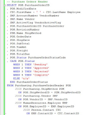
  First things first, even if in a Parent/Child situation as the one of the POs most of the examples deal with reports based on Parent & Chidren information together, it’s a good idea to start understanding first the Parent and then the Child element, in this case the PO Header and then the PO Lines. A query on PO Headers would include also the referenced tables – Vendors, Shipment Methods, Employees, etc. In case of big tables a query would typically include the most important attributes, while from referenced tables are included the most used elements.

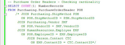
Before further using the query it’s always a good idea to check the variations in cardinality starting from the main table, and increasingly with each join, this test allowing identifying the incorrect joins. When a WHERE clause is involved, it’s easier to use the comment characters (/* … */) and uncomment each join gradually.
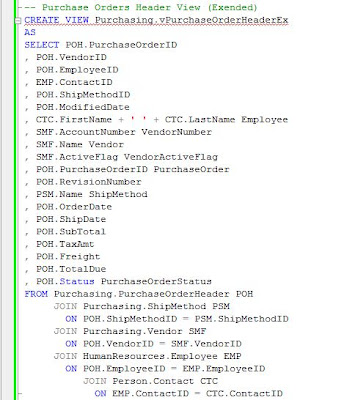
Sometimes it makes sense to encapsulate the query in a view, allowing thus to reuse the logic when needed, minimize maintainability, enforce vertical and horizontal security – to mentioned just a few of views’ benefits. It’s said that views are coming with a slight decrease in performance, though there is always a trade between performance and reusability, including in OOP. It’s recommended to use query writing best practices and target to design your queries for the best performance. Excepting the columns from the initial query, in a view it’s recommended to add also the IDs used in the joins, for faster records filtering or for easier troubleshooting. I prefer to add them in front of the other attributes, though their use could be facilitated when grouped together with the attributes from the table referenced.
Probably you wonder what’s the meaning of Ex postfix, as you probably deducted from the comment, it stands for Extended. In general I prefer to create a view for each level of detail, in this case one for PO Headers and another one for PO Details, and to use nested views when the decrease in performance is minimal, or especially when the views include complex logic I don’t want to replicate. In addition the views could be reused by Users who don’t have to replicate the logic already included in view, making the analysis of data much easier. On the other side, when using views from various modules (e.g. Account Payables vs Pos, Sales vs. Pos), there are many elements which arrive to be used more than once, in general Master Data (e.g. Products, Vendors, Customers, Locations, etc.), thus in order to avoid these type of not necessary joins, I prefer to partition logically the views – two views won’t contain similar data, though this doesn’t mean that won’t be views that contradict this rule.

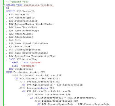
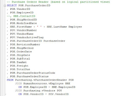
 Using the logical partitioning of views, an alternative view on PO Headers would be created without showing the Vendor end Employee information, following to use if necessary the corresponding views when needed. AdventureWorks includes a view on Vendors called Purchasing.vVendor though the level of detail is at Contact level, and a Vendor could have more than one contacts, therefore the view can’t be used for this purpose, following to create a second view called Purchasing.vVendors (if the name creates confusion you could rename it or rename the Purchasing.vVendor to reflect the fact that the level is Vendor Contacts, for example Purchasing.vVendorContacts).
The problem with the Purchasing.vPurchaseOrderHeaderEx view is that if a user needs additional information about Vendors not available in the view, I’ll have to add the attributes, arriving in the end to create most of the logic available in Purchasing.vVendors view, or the User will rejoin the Purchasing.vVendors view with Purchasing.vPurchaseOrderHeaderEx, having a redundant link to Vendors. The simplified version of the view is the following:
Now the three views - Purchasing.vVendors, HumanResources.vEmployee and Purchasing.vPurchaseOrderHeader could be joined in a query to obtain the same result as Purchasing.vPurchaseOrderHeaderEx view, this approach offering much more flexibility, even if the decrease in performance is higher, though the performance should be in theory better than joining Purchasing.vPurchaseOrderHeader_Ex with Purchasing.vVendors and HumanResources.vEmployee in order to cover the missing attributes. Unfortunately there is another small hitch – the HumanResources.vEmployee view doesn’t contain the ContactID, therefore the view needing to be modified in case is needed.
The logical partitioning allows also more flexibility and relatively increased performance when doing data analysis, for example in order to get the volume purchased per Vendor, the Purchasing.vPurchaseOrderHeader could be used to aggregate the data and join the resulting dataset with Purchasing.vVendors view.
A second look at the same sets of data, Vendors and PO Headers, could be based on a left join between the two, thus seeing also the Vendors for which no PO was approved or completed; the query could be used to return the same data as the previous data set (see ‘Vendors with Pos’ constraint). This second query offers greater flexibility, coming with a small decrease in performance and, in addition, must be taken care of NULL values.
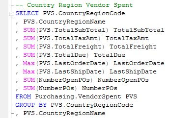
The above examples were showing the cumulated values at Vendor level, what happens when we need to aggregate the data at CountryRegionName level? For this purpose could be used any of the two above queries, and simply aggregate the data at CountryRegionName level. Given the fact that the second query provides greater flexibility, it could be encapsulated in view (e.g. , thus allowing to easily aggregate the data at any level we want – CountryRegionName, StateProvinceName or even City.
 
Sometimes simple aggregations are not enough, Users needing more from the data – for example seeing which is the last/first (open) PO placed in the system for each Vendor. Such a report looks simple as request, though not always so easy to provide. Before the introduction of window functions in SQL Server and analytic functions in Oracle, the techniques for such requests were not so elegant… Here it is the SQL server implementation using RANK ranking window function in order to get the Last/First PO, the same aggregated amounts from the previous query being shown with the help of aggregate window functions.
Note:
Most of the data analysis focuses only for a certain list of vendors, countries or regions, for a certain time interval, or for any other special requirements, for example pending Pos , in order to approximate the future expenses, or for the rejected Pos, in order to see the volume of waste/rework or to quantify the lost opportunities. The above queries were created for general cases and they could be modified for specific requirements if needed.

28 January 2010

SQL Reloaded: Query Writing I (Best Practices)

    In general, when creating queries, the following best practices should be considered:
- Use ANSI-compliant syntax as much as possible.
- Use aliases for all the tables.
- Design for performance reusability and security.
- Reduce unnecessary network traffic.
- Group together the attributes coming from the same table.
- Rename columns in order to avoid confusion, though don’t overreact with this practice.
- Use uniform coding style, formatting and naming conventions
- Use indexed join predicates.
- Learn about the strengths/weaknesses of each feature before using it.
- Use versioning & keep older versions. - Test the queries.
- Write unit tests first [2].
- Handle missing values (NULLs).
- Document database objects inline and specific documents (e.g. Data Dictionaries, Functional Specifications).
- Refactor code
- Use SQL tunings tools.
- Write tiny chunks of code: encapsulate formulas and business logic in functions [2], avoid inline scalar functions.
- Defensive coding: use exception handling, consider all scenarios.


Things to avoid:
- Complex expressions in search conditions [1].
- Join predicates on expressions [1].
- Expressions over columns in local predicated [1].
- Data types mismatches on join columns [1].
- Non-equality join predicates [1].
- Unnecessary outer joins [1].
- Redundant predicates [1].
- Multiple aggregations with DISTINCT.
- Build queries dynamically unless necessary.
- Techniques that use full-table scan: functions that don’t use/perform poor on indexes, wildcards at the beginning of a word.
- Use more attributes/records than needed (particular case: Use * instead of specifying the attributes).
- Using nested views.
- Rely entirely on the code created by wizards and other automation tools.
- UNION unless really needed: use UNION ALL.
- UNIONS instead of conditional-base code (e.g. CASE, DECODE) or self-joins.
- Using temporary tables.
- Server side cursors.
- Procedural queries (e.g. loops, cursors) rather than using set-based queries.
- Redundant logic/code.
- Negations on constraints.
- Code facilitating SQL injection: use parameterized objects.
- Hard-coding values.
- Undocumented functionality.
- Use GROUP BY on final sub-query when it could be used in a sub-query.
- Multiple self-joins/joins to same table instead of GROUP BY.
- Repetitive calls to the same function and same parameters.
- Use constants in ORDER BY clause.
- Create too many versions of the same query.


Note:
    Please note that there are situations and situations, a technique not recommended in general could prove to offer better performance than alternatives (e.g. : recursive simulation + temporary table vs. hierarchical self-joins on SQL Server 2000 ), while for others there are several aspects that need to be considered, for example the trade in performance vs. reusability. Even if most of the database vendors adhere to SQL ANSI standard, in the end each functionality could be implemented differently and vendors could provide additional functionality, therefore could be considered specific best practices for each functionality/vendor.

References: [1] IBM. (????).Best Practice - Writing and Tuning Queries for Optimal Performance [Online] Available from: http://www.ibm.com/developerworks/wikis/display/data/Best+Practice+-+Writing+and+Tuning+Queries+for+Optimal+Performance (Accessed: 27 January 2010)
[2] Oracle. (2009). Cleaning Up PL/SQL Practices, by S. Feuerstein. [Online] Available from: http://www.oracle.com/technology/oramag/oracle/04-mar/o24tech_plsql.html (Accessed: 27 January 2010)

Resources:
Microsoft TechNet. (2010). SQL Server - Best Practices. [Online] Available from: http://technet.microsoft.com/en-us/sqlserver/bb671430.aspx (Accessed: 27 January 2010)

27 January 2010

Business Intelligence: Cognos & SQL Server 2008 - The First Report (Test Drive)

Yesterday evening I installed on my computer the IBM Cognos Express (V9) software, the newest Cognos version, available with a trial period of 30 days. The first attempt to install it was not errorless though as I had to observe several attempts later when I got the same error, the error was not fatal. So, once the instalation complete, the Express Manager started, finding out that I have to install manually the Manager, Advisor, Reporter and Xcelerator - quite easy to do.

Now I was ready to test the tool and create several reports, for this needing to create first a data source - a connection to an existing database with several tables on which the reports will be based. SQL Server 2008's AdventureWorks database seemed to be adequate for this test, in plus I know there are many SQL Server professionals already using it for testing or tutorials.

Step 1: Creating the SQL Server account

Reporting tools need in general only read access to data sources and as a good practice to enforce security and address the special requirements the reports are coming with, so it makes sense to create a new User for this. Open Microsoft SQL Server Management Studio and from the root navigate to Security/New/Login…, this action brining Login – New window in which must be filled

a. the Login name (e.g. cognosuser)
b. the authentification – because Cognos doesn’t supports Windows-based authentication, choose SQL Server authentication, enter the Password and confirm it. By default the ‘Enforce password expiration’ is checked, though this option is not needed for the current requirement so unchek it.
c. Select the Default database, the database you’re intending to base your reports on (e.g. AdventureWorks)
d. Select the ‘Default Language’ (e.g. English)
Navigate to ‘Use Mapping’ tab and in ‘User mapped to this login’ choose the databases you would like to give access (e.g. AdventureWorks) and for each database selected you’ll have to select the schemas in scope (e.g. HumanResources, Person, Production, Purchasing and Sales), while in’Database role membership for’ select the db_datareader database level role name, then you can click ‘Ok’.
 
It’s always a good idea to test the new account before attempting to use it from an external application, this allows catching the eventual issues early in the process, saving your and others’ time!

Step 2: Creating a Data Source

Start the IBM Cognos Express Manager and from Data click on ‘Add…’ button, action that will bring the ‘Enter Data Source Information’ in which you’ll have to select the ‘Data Source Type’, in this case Microsoft SQL Server (SQL 2005 Native Client), fill the ‘Name’ (e.g. AdventureWorks), ‘Server Name’ (here comes your SQL Server name), ‘Database Name’ (e.g. AdventureWorks ), ‘User ID’ (e.g. cognosuser) and password (e.g. something you must guess). As can be seen from the below image, there is also a Databae Object control, which will be populated once you entered the before mentioned information and clicked on ‘Retrieve Database Objects’ button. Select one of the database objects (e.g. AdventureWorks ) and click ‘Ok’, Cognos creating the Data (Source) in the background.
 
Step 3: Creating a Report

Instead of using Report Studio, the standard tool for designing reports, for simple reports or queries could be used instead the Query Studio, an easy-to-use authoring tool, the creation of a report resuming to a simple drag and drop. For this you’ll have to open the Query Studio from the Launch item found on the top menu, this action opening a new browser window, in a next step following to select the package (actually the data source) you want to use. In ‘Insert Data’ mode select a table from the list (e.g. Location) and drag and drop it into the right section, all table’s columns being shown together with a sample set of data.

You could double click on each column and give it a meaningful name – is a good practice to separate the words with spaces though not really necessarily. By clicking on report’s Title you could change its actual value and add a Subtitle if necessary. In ‘Change Layout’ you could change report’s layout by applying different Font, Border and Conditional Styles, much like in Excel, show row numbers by clicking the ‘Show row numbers’ from Change Layout/Set Web Page Size, etc. Save the report once you’ve done the changes, the report will look something like the one from the below image:
Step 4: Running the Report

From ‘Run Report’ Menu item you could choose to run the report mainly in three modes – ‘Run with All Data’, ‘Preview with Limited Data’ or ‘Preview with No Data’. Additionally you can export the report to PDF (Portable Document Format), several versions of Excel (2000, 2002 and 2007), CSV (Comma Separated Values) and XML (eXtensible Markup Language).

Happy coding!

25 January 2010

Data Management: Data Structuredness

Data Management

B. Boehm defined structuredness as 'the degree to which a system or component possesses a definite pattern of organization of its interdependent parts' [1], which transposed to data refers to the 'pattern of organization' that can be observed in data, mainly the format in which the data are stored at macro-level (file or any other type of digital containment) or micro-level (tags, groupings, sentences, paragraphs, tables, etc), emerging thus several levels of structure of different type. From the various sources in which data are stored - databases, Excel files and other types of data sheets, text files, emails, documentation, meeting minutes, charts, images, intranet or extranet web sites, can be derived multiple structures coexisting in the same document, some of them quite difficult to perceive. From the structuredness point of view data can be categorized as structured, semi-structured and unstructured.

In general, at least from my perception, the term of structured data refers to structures that can be easily perceived or known, that raises no doubt on structure’s delimitations. Unstructured data refers to textual data and media content (video, sound, images), in which the structural patterns even if exist they are hard to discover or not predefined, while semi-structured data refers to islands of structured data stored floating with unstructured data. From this perspective, according to [3], database and file systems, data exchange formats are example of semi-structured data, though from a programmers’ perspective the database’s are highly structured, and same for XML files. As also remarked by [2] the terms of structured data and unstructured data are often used ambiguously by different interest groups, in different contexts – web searching, data mining, semantics, etc.

Actually must be done a delimitation between syntactic and semantic aspects of structuredness, the syntactic structuredness referring to 'the rules and patterns formed trough the combination of signs in constructs' [4] in data, while the semantic structuredness to the patterns of meaning, the above definitions applying for both aspects. If we talk about syntax and semantics then most probably it makes sense to talk also about pragmatic structuredness, the third dimension of semiotics. Another reason of confusion is the interchanged use of terms like data, information or knowledge for the same purpose in the same context – see the confusion between data management vs. information management or knowledge management.

Data structuredness is important especially when is considered the processing of data with the help of machines, the correct parsing of data being highly dependent on the knowledge about the data structure, either defined beforehand or deducted. The more structured the data and the more evident and standardized the structure, the easier should be to process the data. Merrill Lynch estimates that 85% of the data in an organization are in unstructured form, most probably this number referring to semi-structured data too. In order to make such data available in a structured format is required an important volume of manual work combined eventually with reliable data/text mining techniques, fact that reduces considerably the value of such data.

Text, relational, multidimensional, object, graph or XML-based DBMS are in theory the most easily to process, map and integrate though that might not be so simple as it looks given the different architectures vendors come with, the fact that the structures evolve over time. In order to bridge the structure and architectural differences, many vendors make it possible to access data over standard interfaces (e.g. ODBC), though there are also systems that provide only proprietary interfaces, making data difficult to obtain in an automated manner. There are also other types of technical issues related mainly to the different data types and data formats, though such issues can be easily overcome.

In the context of Data Quality, structuredness dimension refers to the degree the structure in which the data are stored matches the expectations, the syntactic set of rules defining it. In theory even a minor inadvertence in the structure could lead to processing errors and unexpected behavior. The best example is the one of data available in delimited text files, if any of the character sets used to delimit the structure of the file is available in the data itself, then there are high chances that the file will be parsed incorrectly or the parsing will fail unless the issues are corrected.

References:
[1] Boehm B.W., Brown J.R., Kaspar H., Lipow M., Macleod G.J., Merritt MJ. (1978) "Characteristics of software quality", North-Holland Publishing Company
[2] The Register. (2006) "Structured data is boring and useless", by D. Nortfolk. [Online] Available from: http://www.theregister.co.uk/2006/06/23/unstructured_data/ (Accessed: 24 January 2010)
[3] Wood P. (????) "Semi-structured Data" [Online] Available from: http://www.dcs.bbk.ac.uk/~ptw/teaching/ssd/toc.html (Accessed: 24 January 2010)
[4] Nastase A. (2009) "Utilizing Mind Maps as a Structure for Mining the Semantic Web", Dissertation. University of Liverpool. [Online] Available from: http://www.scribd.com/doc/16612282/Dissertation-paper-Utilizing-Mind-Maps-as-a-Structure-for-Mining-the-Semantic-Web (Accessed: 24 January 2010)

23 January 2010

Data Warehousing: ETL and Synchronization


Data Warehousing

    In a previous post on ETL: SSIS packages vs. SQL code I was mentioning that there are three types of synchronization - of scope, business logic and data, the first targeting to synchronize the filters used to select the data, the second to synchronize the logic used in data processing, when is the case, and third to work with the same unaltered copy of the data.

    The synchronization of scope is achieved by enforcing the same set of constraints to related data elements, usually involving parent-child relations like Invoices Header/ Lines, PO (Purchase Orders) Headers/Lines/Shipments/Distributions, the more general purpose being to keep the referential integrity between the various data elements – assuring for example that all Items appearing in Invoices or POs are in scope or that all Invoice Lines have the corresponding Invoice Headers, and vice-versa.

    The synchronization of business logic could be for example enforced for data sets coming from distinct systems, usually involving different architecture, or for data sets requiring similar logic, considering the cases when data needs to be duplicated with slightly differences; the simplest example I can recall from the later category being the creation of Item Master Data for the existing Inventory Organizations, the respective data sets needing to be created before the data are actually loaded.

    The synchronization of data requires working with the same unaltered data in the various threads of processing, either packages or SQL code; it’s quite simple as concept, though not always straightforward to achieve. For this purpose it makes sense to load the data in the local database, even for slowly changes data sources like data warehouses, and base the business logic on the respective local data set(s) rather than loading the data over and over again for each package, this involving also considerable additional network traffic. Why the alternative is not the best approach? 
Supposing that two packages A and B are scheduled to run at the same time, even if the requests are sent simultaneously to the database, the simultaneously is relative, because most of the time the requests are queued, in general following to be processed in the order they came, though this depends on legacy system’s architecture and settings. 
Supposing that there is some time elapsed between the times the two requests are processed, there are good chances that one record was created, deleted or updated in between. The impact of changes in data could be minimum though unpredictable situations might result with unpredictable impact. There are chances to find the issue when loading the data in the destination system, this if adequate validation is performed by it, though there are good chances to load the without noticing anything, the issues being eventually discovered later. 

    It should be targeted to cover all three types of synchronization even if it complicates the design more than expected, though I think it’s better to do defensive architecting/programming, the increase in complexity being relative if we’re considering the plumbing/redesign that needs to be done in order to fix the issues.

Data Warehousing: ETL (SSIS packages vs. SQL code)

Data Warehousing

I’ve been working with DTS (Data Transformation Services) packages for the past 7-8 years, finding SQL Server’s 2000 functionality pretty useful in handling ETL (Extract, Transform, Load) tasks, especially when importing and exporting data between multiple data sources. The functionality provided by the DTS platform was basic, though it could be extended in custom packages with code developed in VB or by using ActiveX tasks in VBScript/Jscript, when the SQL-based logic was not enough. In addition, all three types of coding could make calls to .dlls, and thus operating system, vendor or in-house built libraries or simple functions could be (re)used. 

Starting with SQL Server 2005, DTS was replaced by the SSIS (SQL Server Integration Services) component, becoming with SSRS (SQL Reporting Services) and SSAS (SQL Server Analysis Services) integrant part of Microsoft's data platform. Besides providing a new architecture, SSIS extended the functionality previously available, bringing more flexibility in constructing the packages, their elements and data manipulation. SSIS became with each new version of SQL Server (2008, 2012, 2014, 2016, 2017, 2019) a powerful ETL tool that can be easily used for Data Warehousing, Data Migration or Data Integration projects. 

In what concerns ETL we could say there are two main philosophies - have as much of the business logic in the (ETL) package, or use the package mainly for loading data from the various sources and have the business logic in the database as SQL-based code. As always, each of the two philosophies has its own advantages and disadvantages, though I would consider a third philosophy – design for performance, reuse and maintainability, resulting thus a hybrid between the first two mentioned philosophies. 

There are several other factors that need to be considered when building ETL solutions - synchronization, testability, security, stability, scalability, complexity, learning curve, etc. I would say that there is no perfect receipe, no architecture matching all requirements, each solution coming with its needs and constraints, sometimes being a good idea to go one level of abstraction above the requirements, while other times is better to stick to the requirements and problem at hand. 

Performance

Designing for performance resumes in choosing the architecture/methods that provides the best performance individually and as a whole – either using package-based functionality, SQL-based functionality or a combination of both. In general SQL code is best suited for query-based data manipulation, while packages are better suited for sequential or workflow-based processing of data, though there could be exceptions and exceptions. Often it’s a good idea to test the performance of all alternative approaches via a prototype, even if in time the developer arrives to a good knowledge of the methods that suit best from a performance point of view.

Reuse

Each of the two architectures allow a lower or higher degree of reuse using parameters, variables and compartmenting of code, maybe with a plus for SQL code which has in theory a greater maturity and flexibility than the package-based functionality, allowing a wider range of reuse resulted from the compartmenting of code in the various supported objects (stored procedures, functions, views or tables).

Maintainability

Maintainability, the easiness of modifying packages or code, is an important factor because few are the cases in which the logic doesn’t change over time, many projects having to deal with change in requirements, sometimes implying a 180 degrees change of the overall perspective. Therefore it's important to be able to modify the code/package and even change the architecture with a minimum of effort.

Refactoring

Refactoring resumes in modifying the code without changing the functional behavior in order to improve the performance, readability, maintainability or extensibility, minimize the use of resources, remove redundant code, adhere to standards, best practices or naming conventions. It is said that there is always place for improvement, performance being the dimension with the most important impact in the world of databases. Refactoring is not always necessary, though it’s a good practice for achieving high quality solutions.

Synchronization

I would say there are three types of synchronization – of scope, business logic and data, the first targeting to synchronize the filters used to select the data, the second to synchronize the logic used in data processing, when is the case, and third to work with the same unaltered copy of the data. Considering the example of Invoices – Headers and Lines, the synchronization of scope would resume to apply the same constraints for the two, assuring that there is no Invoice Header without Lines, and vice-versa; the data synchronization between the two referring to the fact that the data between the two data sets should be consistent, there should be no change in Invoice Headers not reflected also at Line level (e.g. total amount matching between Lines and Header). Business logic synchronization refers typically to the use of the same set of data for similar purposes, if several transformations were used for Invoice Headers, they should be reflected accordingly also at Invoice Line level. Synchronization it’s actually quite an important topic, therefore I will reconsider it in a further post.

Testing & Troubleshooting

I find that the business logic implemented in SQL code is much easier to test than the logic implemented in packages, because in the first situation each object and step could be in theory tested individually/progressively, being thus much easier to troubleshoot. Troubleshooting packages logic can be quite complex because is not always possible to view the input/output for each intermediary step.

Complexity

Complexity is reflected in the easiness of understanding the logic broken down to pieces and as a whole. Packages are highly visual, being in theory easier to identify and understand the steps and their flow, even by non-technical people, while SQL-code might need auxiliary representations for the same purpose (e.g. data flow diagram) and need a higher level of expertize. 

Security

Security is always a sensitive and complex topic, and in general it resumes to how secure is the code and sensitive information stored (e.g. user name & password, data), who has access to execute it and the context in which the code is run. This can become easily quite a complex topic, being highly dependent on the architecture used.

Stability

We can discuss about platform and design stability, which can be often a matter of perception and experience. Both SSIS and database engines could be considered as stable development environments, the later having in theory a greater maturity and flexibility, flexibility that could be easily brought to extreme creating bad coding monsters (e.g. loop calls to .dll libraries), impacting thus design’s stability, which is correlated to the adequate use of functionality, techniques and resources – each technology has its does and don’ts, strength and weakness.

Deployment
 
Deployment of business logic on the server can be quite easy or quite complex, depending on the overall architecture, the number of configurable items in scope, and the complexity of the dependencies existing between them. The deployment usually resumes at copying the code from one location to another, installing the eventual dependencies and configuring the objects for use.

Scalability

Scalability in this context refers mainly to the degree the business logic can cope with the increased volume of records, and not necessarily with the number of requests, though this aspect could be considered too, after case. SSIS and the database engines are designed to be highly scalable, though there are architectures and architectures, good uses and misuses of techniques. Designing for performance in theory equates with good scalability, unless the requirements makes it difficult to have a scalable solution.

Learning curve

The learning curve of technologies is always an important factor that needs to be considered in development, as it reflects how much time an average developer needs to master the basic/average/complex functionality provided by the respective technology. For ETL development is in general requested an average knowledge of both - SSIS architecture, respectively SQL-based programming - though it’s not easy to acquire both problem-solving mindsets. A SSIS developer usually attempts using as much as possible the functionality provided by SSIS, while a SQL developer the SQL-based functionality. In the end, it’s important to know how to balance between the two.

Previous Post <<||>> Next Post

19 January 2010

Business Intelligence: Levels of Accuracy in Reporting

Business Intelligence

Correlated with the level of detail (aka granularity), another aspect that needs to be considered in reports is results’ levels of accuracy – how much the data reflect the reality at each level of detail. Because the integration between modules of the same or different systems brought some of the attributes from one module into the other (e.g. Document Numbers, UIDs, Dates), the reports can consider the respective attributes in queries without involving the modules they come from. Thus for example in order to create an AP (Account Payables) Invoices report, could be sufficient to use the GL (General Ledger) Date stored in AP without using the GL data directly; on the other side, a more accurate report is obtain when using the AP and GL data, such a report could include also the manual postings made in GL and not available in AP. 

Typically the data from one module that are stored in other modules, should be in synch, though there could be exceptions and exceptions. In the end it is developer’s task to understand the level of accuracy/detail the users need; in general it doesn’t always make sense to provide the highest level of accuracy/detail when the user needs only some rough number, as higher level of accuracy/details equate with more effort and more tables added to a report.

When considering the different levels of accuracy/detail within reports, given two modules/entities A and B, we might end up created a set of reports with:
a.  all records from A
b.  all records from B;
c.  all records from A and matching records from B, and vice-versa;
d.  all records from A and aggregated data from B when the level of detail is changed.
e.  aggregated data from A vs. aggregated data from B in case of many-to-many cardinality, the aggregation being made at a level of detail in which the amounts are not duplicated.
f.  mismatches between A and B for the same scope (it can be shown at different levels of details).

These scenarios would allow Users to choose the report with the needed level of detail/accuracy, though covering all existing scenarios could be quite expensive, not to neglect the fact that there are reports spanning more than 2 modules. On the other side, two reports for A and B would be sufficient as long as the reference attributes between modules are provided, falling in Users’ task to match and aggregate the data, though also this alternative could prove to be problematic because of the volume of data, synchronization issues between data sets or lack of adequate skill set, and all related issues. The first solution is the ideal, the second is workable, though in the end it depends what makes the users happy.

Previous Post <<||>> Next Post

Data Quality Dimensions: Consistency (Definitions)

"The degree of uniformity, standardization, and freedom from contradiction among the documents or parts of a system or component."  (IEEE," IEEE Standard Glossary of Software Engineering Terminology", 1990)

"Describes whether or not master data is defined and used across all IT systems in a consistent manner. For example, do all systems have the same Customer address? continuous availability The combination of high availability and continuous operations, thus addressing all categories of outages." (Allen Dreibelbis et al, "Enterprise Master Data Management", 2008)

"The requirement that a transaction should leave the database in a consistent state. If a transaction would put the database in an inconsistent state, the transaction is canceled." (Rod Stephens, "Beginning Database Design Solutions", 2008)

"Describes whether or not master data is defined and used across all IT systems in a consistent manner. For example, do all systems have the same Customer address? continuous availability The combination of high availability and continuous operations, thus addressing all categories of outages." (Martin Oberhofer et al, "Enterprise Master Data Management", 2008)

"The degree to which one set of attribute values match another attribute set within the same row or record (record-level consistency), within another attribute set in a different record (cross-record consistency), or within the same record at different points in time (temporal consistency)." (DAMA International, "The DAMA Dictionary of Data Management" 1st Ed., 2010)

"Consistency is a dimension of data quality. As used in the DQAF, consistency can be thought of as the absence of variety or change. Consistency is the degree to which data conform to an equivalent set of data, usually a set produced under similar conditions or a set produced by the same process over time." (Laura Sebastian-Coleman, "Measuring Data Quality for Ongoing Improvement ", 2012)

"The degree to which data values are equivalent across redundant databases. With regard to transactions, consistency refers to the state of the data both before and after the transaction is executed. A transaction maintains the consistency of the state of the data. In other words, after a transaction is run, all data in the database is 'correct' (the C in ACID)." (Craig S Mullins, "Database Administration", 2012)

"Agreement of several versions of the data related to the same real objects, which are stored in various information systems." (Boris Otto & Hubert Österle, "Corporate Data Quality", 2015)

"Consistency: agreement of several versions of the data related to the same real objects, which are stored in various information systems." (Boris Otto & Hubert Österle, "Corporate Data Quality", 2015)

"The degree to which the data reflects the definition of the data. An example is the person name field, which represents either a first name, last name, or a combination of first name and last name." (Piethein Strengholt, "Data Management at Scale", 2020)

"The degree to which the model is free of logical or semantic contradictions." (Panos Alexopoulos, "Semantic Modeling for Data", 2020)

"The degree of uniformity, standardization, and freedom from contradiction among the documents or parts of a component or system." [IEEE 610]

18 January 2010

Data Quality Dimensions: Referential Integrity

  
Data Management

In relational databases’ world there are three types of integrity mentioned – entity, referential and domain integrity. Entity integrity demands that all the tables must have a primary key that contains no Null values, the referential integrity demands that each non-null value of a foreign key must match the value of a primary key [1], while the domain integrity demands that the type of an attribute should be restricted to a certain data type, the format should be restricted by using constraints, rules or range of possible values [2]. 
Even if not mandatory, all three types of integrity are quintessential for reliable relational databases, with a plus for referential integrity. When the referential integrity is not enforced at database level or at least in code, then it might happen that a record from a table is deleted and a foreign key it’s still pointing to it, fact that could lead to unexpected disappearance of records from system’s screens even if the records are still in the database. 

During conversions or data migrations is important to assure that the various sets loaded match the referential and domain integrity of the database in which the data will be loaded, otherwise the records not respecting the mentioned type of integrity will be rejected. The rejection itself might not be a problem for several records, though when it happens at large scale, then the situations changes dramatically, especially when the system gives no adequate messages for the cause or rejection. A good approach for such scenarios is to assure that the scope is synchronized between the various data elements, and that the referential integrity of datasets is validated before the data are loaded in the destination database.

Note:
Expect the unforeseeable! It’s always a good idea to check whether the referential integrity is kept by a system – there are so many things that could go wrong! There are even systems (e.g. data warehouses) that don’t necessarily need referential integrity, though in time that might become quite a problem, therefore it’s a good idea to have in place mechanisms that check for this kind of issues.

References:
[1] Halpin. T. (2001) Information Modeling and Relational Databases: From Conceptual Analysis to Logical Design. Morgan Kaufmann Publishers. ISBN 1-55860-672-6.
[2] MSDN. 2009. Data Integrity. [Online] Available from: http://msdn.microsoft.com/en-us/library/ms184276.aspx (Accessed: 18 January 2009)

Data Quality Dimensions: Consistency

Data Management

Consistency refers to the extent values are consistent in notation, this often supposing the existence of a predefined list of values (LOV), a data dictionary, an ontology or any other type of knowledge representation form (e.g. charts, diagrams) that can be used to 'enforce' data consistency. Enforce is maybe not the best term to describe the state of art because the two data sets could be disconnected from each other, being in Users’ responsibility to ensure the overall consistency, or the two data sets could be integrated using specific techniques. In most of the cases is checked the consistency of the values taken by one attribute against an existing LOV, though for example for data formed from multiple segments (e.g. accounts) each segment might need to be checked against a specific data set or rule generator , such mechanisms implying multi-attribute mappings or associational rules that specify the possible values.

Consistency could be in general considered against two distinct data sets or distinct systems, typically one of them functioning as master, between records (record-level consistency), between a set of attributes from different records (cross-record consistency) or within the same record but at different points in time (temporal consistency) [3]. It makes sense to talk about consistency especially in regard to master data, being important to keep the consistency of one or more attributes in the various systems against the master data.

As highlighted also by [1], there are two aspects of consistency: the structural consistency in which two or more values can be distinct in notation but have the same meaning (e.g. missing vs. n/a), and semantic consistency in which each value has a unique meaning (only n/a for example is allowed in order to highlight missing values). It should be targeted to have the data semantically consistent, in order to avoid confusions, accidental exclusion of data during filtering or reporting. More and more organizations are investing in ontologies, they allowing ensuring the semantic consistency of concepts/entities, though for most of the cases simple single or multi-attribute lists of values are enough.

There are several sources (e.g. [2]) that consider Codd’s referential integrity constraint as a type of consistency, in the support of this idea could be mentioned the fact that referential integrity could be used to solve data consistency issues by bringing the various LOV in the systems, though I would prefer to separate the two concepts because referential integrity is mainly an architectural concept even if it involves the 'consistency' of foreign key/primary key pairs.

References:
[1] Chapman A.D. (2005) "Principles of Data Quality", version 1.0. Report for the Global Biodiversity Information Facility, Copenhagen
[2] Lee Y.W., Pipino L.L., Funk J.D., Wang R.Y. (2006) "Journey to Data Quality", MIT Press. ISBN: 0-262-12287-1.
[3] David Loshin (2009) Master Data Management. Morgan Kaufmann OMG Press. ISBN 978-0-12-374225-4.

Data Quality Dimensions: Accuracy (Definitions)

"(1) A qualitative assessment of correctness, or freedom from error. (2) A quantitative measure of the magnitude of error." (IEEE, "IEEE Standard Glossary of Software Engineering Terminology", 1990)

[accuracy (of measurement):] "Closeness of the agreement between the result of a measurement and a true value of the measurand." International Vocabulary of Basic and General Terms in Metrology, 1993)

"A qualitative assessment of freedom from error or a quantitative measure of the magnitude of error, expressed as a function of relative error." (William H Inmon, "Building the Data Warehouse", 2005)

"A data element’s degree of conformity to an established business measurement or definition. Data precision is the degree to which further measurements or definitions will show the same results." (Jill Dyché & Evan Levy, "Customer Data Integration: Reaching a Single Version of the Truth", 2006)

"Degree of conformity of a measure to a standard or a true value. Level of precision or detail." (Martin J Eppler, "Managing Information Quality" 2nd Ed., 2006)

"The accuracy reflects the number of times the model is correct." (Glenn J Myatt, "Making Sense of Data: A Practical Guide to Exploratory Data Analysis and Data Mining", 2006)

"An aspect of numerical data quality connected with a standard statistical error between a real parameter value and the corresponding value given by the data. Data accuracy is inversely proportional to this error." (Juliusz L Kulikowski, "Data Quality Assessment", 2009)

"An inherent quality characteristic that is a measure of the degree to which data agrees with an original source of data (such as a form, document, or unaltered electronic data) received from an acknowledged source outside the control of the organization." (David C Hay, "Data Model Patterns: A Metadata Map", 2010) [accuracy in regard to a surrogate source]

"An inherent quality characteristic that is a measure of the degree to which data accurately reflects the real-world object or event being described. Accuracy is the highest degree of inherent information quality possible." (David C Hay, "Data Model Patterns: A Metadata Map", 2010) [accuracy in regard to reality]

"Freedom from mistakes or error, conformity to truth or to a standard, exactness, the degree of conformity of a measure to a standard or true value. (Michael Brackett, 2011)

"The degree to which a data attribute value closely and correctly describes its business entity instance (the 'real life' entities) as of a point in time." (DAMA International, "The DAMA Dictionary of Data Management", 2011)

"Accuracy is the quality or state of being correct or precise; accurate information is correct in all details (NOAD)." (Laura Sebastian-Coleman, "Measuring Data Quality for Ongoing Improvement ", 2012)

"Within the quality management system, accuracy is an assessment of correctness." (For Dummies, "PMP Certification All-in-One For Dummies" 2nd Ed., 2013)

"How closely a measurement or assessment reflects the true value. Not to be confused with precision [...]" (Kenneth A Shaw, "Integrated Management of Processes and Information", 2013)

"Accuracy is defined as a measure of whether the value of a given data element is correct and reflects the real world as viewed by a valid real-world source (SME, customer, hard-copy record, etc.)." (Rajesh Jugulum, "Competing with High Quality Data", 2014)

"Within the quality management system, accuracy is an assessment of correctness." (Project Management Institute, "A Guide to the Project Management Body of Knowledge (PMBOK® Guide)" 6th Ed., 2017)

"The degree to which the data reflect the truth or reality. A spelling mistake is a good example of inaccurate data." (Piethein Strengholt, "Data Management at Scale", 2020)

"The degree to which the semantic assertions of a model are accepted to be true." (Panos Alexopoulos, "Semantic Modeling for Data", 2020)

"Closeness of computations or estimates to the exact or true values that the statistics were intended to measure." (SDMX) 

"The capability of the software product to provide the right or agreed results or effects with the needed degree of precision." [ISO/IEC 25000]

 "The closeness of agreement between an observed value and an accepted reference value." (American Society for Quality)

"The term “accuracy” refers to the degree to which information accurately reflects an event or object described." (Precisely) [source]

17 January 2010

Data Quality Dimensions: Accuracy

Data Management

Accuracy refers to the extent data are correct, match the reality with an acceptable level of approximation. Correctness, the value of being correct, same as reality are vague terms, in many cases they are a question of philosophy, perception, having a high degree of interpretability. However in what concerns data they are typically the result of measurement, therefore a measurement of accuracy relate to the degree the data deviate from physical laws, logics or defined rules, though also this context is a swampy field because, utilizing a well-known syntagm, everything is relative. 
From a scientific point of view we try to model the reality with mathematical models which offer various level of approximation, the more we learn about our world, the more flaws we discover in the existing models, it’s a continuous quest for finding better models that approximate the reality. Actually, things don’t have to be so complicated, for basic measurements there are many tools out there that offer acceptable results for most of the requirements, on the other side, as requirements change, better approximations might be required with time.

Another concept related with the ones of accuracy and measurement systems is the one of precision, and it refers to degree repeated measurements under unchanged conditions lead to the same results, further concepts associated with it being the ones of repeatability and reproducibility. Even if the accuracy and precision concepts are often confounded a measurement system can be accurate but not precise or precise but not accurate (see the target analogy), a valid measurement system targeting thus both aspects. This being said accuracy and precision can be considered dimensions of correctedness.

Coming back to accuracy and its use in determining data quality, typically accuracy it’s strong related to the measurement tools used, for this being needed to do again the measurements for all or a sample of the dataset and identify whether the requested level of accuracy is met, approach that could involve quite an effort. The accuracy depends also on whether the systems used to store the data are designed to store the data at the requested level of accuracy, fact reflected by the characteristics of data types used (e.g. precision, length).

Given the fact that a system stores related data (e.g. weight, height, width, length) that could satisfy physical, business of common sense rules, could be used rules to check whether the data satisfy them with the desired level of approximation. For example being known the height, width, length and the composition of a material (e.g. metal bar) could be determined the approximated weight and compared with entered weight, if the difference is not inside of a certain interval then most probably one of the values were incorrect entered. There are even simpler rules that might apply, for example the physical dimensions have to be positive real values, or in a generalized formulation - involve maximal or minimal limits that lead to identification of outliers, etc. In fact most of the time determining data accuracy resumes only at defining possible value intervals, though there will be also cases in which for this purpose are built complex models and used specific techniques.

There is another important aspect related to accuracy, time dependency of data – whether the data change or not with time. Data currency or actuality refers to the extent data are actual. Given the above definition for accuracy, currency could be considered as a special type of accuracy because when the data are not actual then they don’t reflect the reality. If currency is considered as a standalone data quality dimension, then accuracy refers only to the data that are not time dependent.

Business Intelligence: Levels of Detail in Reporting

Business Intelligence

Working with data mainly from frontend (User Interface), in general Users have limited knowledge on how the data are physically stored in the various systems existing in an organization. When a new report is needed they point out the attributes they know from the screens they are working with, falling in developers’ duties to figure out whether the “soup of attributes” makes really sense and find a workable solution. Once the developer has identified the attributes and the tables they are stored in, he/she can go on and create the query/queries on which the report will be based upon. For this task is important to know how the various tables relate to each other, in other words knowing the attributes which can be used to link the tables or which is the relational path to link the table, and relations’ cardinality, which reflects how the number of records of a table or data set changes when is joined with another table or data set.

Between two tables and extensively two data sets the relations could have any of the four types of cardinality – many-to-many (represented as m:n), one-to-one (1:1), one-to-many (1:n) and the reverse many-to-one (n:1). It could be given a definition for each of the cardinality types, though it’s easier to remember that in the x-to-y compounds, between two tables or data sets A and B, x has the value ‘one’ when the number of references from table B to any record from A is maximum 1 (there could be records not referenced at all), and ‘many’ when at least a record could be referenced more than once; the same logic applies for y but inversing the tables’ perspective.

The level of detail (LOD) of a report (aka data granularity) is directly correlated with the changes in cardinality - by adding a data set to an existing data set, if the cardinality of one-to-many and many-to-many is implied then the level of detail changes too. In other words if a record in a given data set is referenced more than once in the new added table then the LOD changes. A simple example of change of LOD occurs in parent-child/master-details relations. For example if the Invoice Lines are added to a data set based on Invoice Header then the LOD changes from Invoice Headers to Invoice Lines. If the Payments are added to the resulted data set then the LOD changes from Invoice Lines to Payments only if there are multiple Payments for an Invoice (one-to-many or many-to-many cardinalities), otherwise LOD remains the same.

Summarizing, the level of detail of a report is the lowest level at which a cardinality change occurs at entity level. It can be discussed about lower or higher LOD in relation to a given level of detail, for example Invoice Payments have a lower LOD than Invoice Lines, while Invoice Header a higher LOD.

Why is it necessary to introduce the LOD especially when considering a relatively complex notion as cardinality?! It worth defining it mainly because the term is used when defining/mitigating reporting requirements, its use being intuitive rather than well-defined and understood. When creating reports it’s important to find the adequate LOD for a report and know what methods can be used in order to pull data that would normally change reports’ LOD without actually changing reports’ LOD.

The limitations imposed by the need to report at a certain LOD higher than the one implied by the row data can be overcome with the help of aggregate functions used with GROUP BY constructs. Such constructs make it possible to bring into a report data found at lower LOD than the reporting LOD by grouping the data based on a set of attributes. The aggregate functions provide functionality to calculate for a set of values the maximum, minimum, sum, count of records, standard deviation, and other statistical values, all of them working on numeric data types, while maximum/minimum and count of records work also with dates or alphanumeric data types.

For example using aggregate functions the Invoice amounts can be aggregated and shown at Invoice Header level, however, in contrast, it’s not possible to do the same with quantities, because typically each Invoice Line refers to a specific Product, and as apples can’t be counted with peaches, this means that in order to see the quantities, the level of detail has to be changed from Invoice Header to Invoice Line. The same technique could be applied to similar parent-child (master-details) relations covering one-to-many or one-to-one cardinality, and also many-to-many relations that involve higher reporting complexity.

Direct many-to-many relations are seldom, involving mainly data sets, the attributes used in relation appearing more than once in each dataset (at least once). Taking an example from ERP world, there could be multiple Receipts and Invoices for the same Purchase Order, thus if there is no direct match between Receipts and Invoices to identify uniquely which Invoice belong to each Receipt, a report involving all the three entities could be barely usable, records being duplicated (e.g. 2 Invoices vs. 3 Receipts result in 6 records in a such scenario). For such reports to be usable the LOD needs to be change at a higher level at least on one side, thus reconsidering the mentioned example a report could show the Purchase Order details and aggregating the Invoice & Receipt Quantities/Amounts at Purchase Order level, or show detailed Invoices with aggregated Receipt information, respectively detailed Receipts with aggregated Invoice information.

Unfortunately even if the aggregate functions are quite handy they have their own limitations, being difficult to use them in order to answer to questions like “what was the last product sold for each customer”, “which was latest invoice placed for each customer”, at least not without considerable effort from developer’s side. Fortunately database vendors implemented their own more specialized type of aggregate functions - analytic functions in Oracle and window functions in SQL Server, they allowing modeling such questions with a report. The downside for developers is that each database vendor comes with its own philosophy, so techniques and features working in one database might not work in another.

15 January 2010

Data Warehousing: Dimension Hierarchy (Definitions)

"An arrangement of members of a dimension into levels based on parent-child relationships, such as Year, Quarter, Month, and Day or Country, Region, State or Province, and City. Members in a hierarchy are arranged from more general to more specific." (Microsoft Corporation, "SQL Server 7.0 System Administration Training Kit", 1999)

"A navigation path that allows the user to move from summarized to detailed information with each level of the hierarchy represented by a different attribute." (Reed Jacobsen & Stacia Misner, "Microsoft SQL Server 2005 Analysis Services Step by Step", 2006)

"A series of master-detail relationships within a dimension. Many front-end tools require hierarchy definitions in order to support drilling features. Some aggregate navigation and construction tools, such as Oracle's materialized views, require explicit declaration of a hierarchy if a dimension is to be partially summarized by an aggregate fact table." (Christopher Adamson, "Mastering Data Warehouse Aggregates", 2006)

"A logical tree structure that organizes the members of a dimension such that each member has one parent member and zero or more child members." (Microsoft, "SQL Server 2012 Glossary", 2012)

14 January 2010

Data Quality: Data Cleansing

    Even if often Data Cleansing or Data Scrubbing is considered synonymous to Data Cleaning, it actually includes the Data Validation and Data Cleaning process, where Data Validation is the process of checking data quality against a set of rules (referred as data quality rules) in a given set of data, and Data Cleaning or Data Correction is the process of correcting the data quality issues identified in Data Validation. Data Cleansing consists in general of the following steps:

Step 1: Defining the scope

    The scope definition resumes at the identification of elements, attributes and the records that need to be cleaned. If is intended only to improve overall data quality and nothing else, the focus will be mainly on the data elements and attributes perceived as having low data quality. For data conversion the elements in scope are defined based on the requirements of the destination system and overall business requirements are defined the attributes in scope, an exercise that needs to be performed is the data mapping between the destination on one side and the legacy system(s) and the other data sources (e.g. Excel, MS Access files) on the other side.

    From case to case in scope for cleansing might be all the records available in the legacy system(s) for a given set of data elements and attributes, or only a fraction of them, usually the focus is mainly the active and open records, and eventually some historical records. By active records are referred those records not cancelled or disabled, either master and transactional data , by open records the (transactional) records not marked as closed, records on which an action is still pending (e.g. pending Invoice Receipt, Payment, etc.), while by historical records are referred the already closed transactional data (e.g. Purchase Orders, Sales Orders, etc.).

    Given the importance of master data for the business they are often the starting point for cleaning, they being also the data elements with the longest issue resolution, the transactional data being in theory easier to clean. The two types of data need to be synchronized the referent data related to the transactional data in scope needs to be loaded too.

Step 2: Defining the data quality rules and error types.

    The data quality rules are defined for the attributes in scope and the data quality dimensions considered that apply, typically data accuracy, completeness, conformity, consistency, duplication and referential integrity. The issues are eventually further categorized and prioritized.

Step 3: Validating the data quality rules

    The data quality rules are validated against the actual data sets, the output of the rules are consolidated in reports that follow to be interpreted. The number of errors are reported and stored for historical trending in case several iterations are needed for data cleaning.

Step 4: Identifying the data quality issues.

    The reports are reviewed by the data owners, the issues being identified and the rules validated, further steps being performed in order to identify the root causes for the discovered issues. This usually leads to the calibration of data quality rules as new scenarios (e.g. exceptions, new error types) can be discovered.

Step 5: Correcting the data quality issues.

    The issues are mitigated and corrected, issues’ resolution time, the time needed to correct the issues, is directly dependent on the volume of issues, their complexity, the number of resources allocated to the task, on whether the issues are corrected in the source or on a copy of the data, on whether the cleansing is done manually or specific software tools are used. Specific Data Cleaning software tools can help decreasing considerably the volume of manual work involved during the process, being preferred to use automatic and semiautomatic data cleansing methods whenever is possible.

Step 6: Validating the changes against the same data quality rules.

    Once the issues are corrected the data sets are validated against the same rules used at Step 3, the Steps 3 to 5 being repeated until the expected data quality level is achieved. As already highlighted in a previous post, Data Cleansing is not a one-time endeavor, but an iterative process, new iterations being requested by changes occurred in rules or in scope, by the sequencing/scheduling of cleansing work or by reporting frequency (centered or not along the important milestones).

Step 7: Documenting/Reporting error results and validation outcomes, if needed.

    Starting with data elements, attributes, and the logic used to select the records in scope for cleaning, and ending with the data quality reports with the issues and the improvement trends it makes sense to document everything and summarize it in a set of best practices and lesson learned sessions.

Step 8: Modify processes/procedures to reduce issues occurrence.

    There are chances to discover that the errors found during validation could be avoided by modifying the existing processes, procedures or standards, or enforcing new validation rules in the legacy systems. When the changes are complex might be started even individual projects to address them.
Related Posts Plugin for WordPress, Blogger...

About Me

My photo
IT Professional with more than 24 years experience in IT in the area of full life-cycle of Web/Desktop/Database Applications Development, Software Engineering, Consultancy, Data Management, Data Quality, Data Migrations, Reporting, ERP implementations & support, Team/Project/IT Management, etc.